2017-07-21

[0024] Iterative Closest Points（迭代最近点）

ICP 算法简介

由点云配准 说起

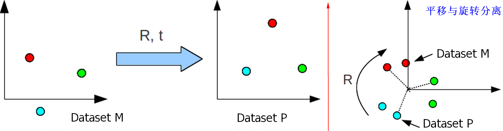
　Point cloud registration, is the process of finding a spatial transformation that aligns two point clouds. The purpose is to merge point clouds of multiple views into a globally consistent model.
　Iterative Closest Points (ICP) is an algorithm employed to minimize the difference between two clouds of points. In the algorithm, target point cloud, is kept fixed, while the other one, the source, is transformed to best match the reference (the target). The algorithm iteratively revises the transformation (combination of translation and rotation) needed to minimize the distance from the source to the reference point cloud.
问题描述
- 有两个点集，source 和 target，target 不变（前一帧点云），source（当前帧）经过旋转（rotation）和平移（translation）甚至加上尺度（scale）变换，使得变换后的 source 点集尽量和 target 点集重合，这个变换的过程就叫 点云配准。
  
  Input：$M$，$P$
  Output：rotation $R$，translation $T$，s.t. $min \verb|{| dist(M’, P) \verb|}|, \space M’ = R * M + T$
- ICP 是最广泛应用的配准方法，ICP 利用迭代一步步地算出正确的对应关系。

经典的ICP算法

1992年，Paul J.Besl and Neil D.Mckay 在他们的文章《A method for Registration of 3D Shape》中提出了ICP（Iterative closest point）算法，通过迭代、寻找来不断搜索最近点，定义一个阀值（threhold）最终完成多视图的拼合。在那个年代提出这一划时代的算法，是不可思议的，其中很多思路没有一定的数学功底和站在一个相当的高度是难以实现的：
- 将点集差异转换成协方差矩阵，然后通过奇异值 SVD 分解求最大特征向量；
- 最大特征向量对应四元数即为其欧式运动对应值，完成数据拼合。
ICP Algorithm
- ①Start from initial guess
- ②Iterate（最大迭代次数）
  - 2.1 For ecah point $M_i$，find closest point $P_i$
  - 2.2 Find best transform for this correspondance
  - 2.3 Transform M

基本原理

两个点集 $M$、$P$ 中的点数不一定相同，给出两个点集的空间变换 $f$ 使它们能进行空间匹配；$f$ 是一未知函数，求解 $f$ 的这个问题使用的最多的方法是迭代最近点法（Iterative Closest Points Algorithm）。
ICP 基本思想是：根据某种几何特征对数据进行匹配，并设这些匹配点为假想的对应点，然后根据这种对应关系求解运动参数；再利用这些运动参数对数据进行变换；利用同一几何特征，确定新的对应关系，重复上述过程。
- 第①步：计算 $M$ 中的每一个点在 $P$ 中的对应近点
- 第②步：求得使上述对应近点对平均距离最小的刚体变换（平移矩阵+旋转矩阵）
- 第③步：对 $M$ 使用上一步求得的平移矩阵和旋转矩阵，得到新的变换点集 $M’$
- 第④步：如果新的变换点集 $M’$ 与参考点集 $P$ 满足收敛条件，则停止迭代计算；否则，变换点集 $M’$ 作为新的 $M$ 继续迭代第①～③步，直到达到收敛条件。
  - Converges（是否收敛？）
    - Errors decrease monotonically（偏差单调减少）
    - Converges to local minimum（陷入局部最优解）
    - Good initial guess $\Longrightarrow$ Converges to global minimum（全局最优解）
  - 收敛条件
    - 前一个变换矩阵和当前变换矩阵的差异小于阈值时，认为已经收敛
    - 均方误差和（Mean Square Error, $\sigma = \sqrt{\frac{\sum ^n \varepsilon _i ^2}{n}}$）小于阈值

ICP 目标函数

三维空间中两个 3D 点，$\overrightarrow{M_i} = (x_i, y_i, z_i)$，$\overrightarrow{P_j} = (x_j, y_j, z_j)$，它们的欧氏距离表示为：$$dist(\overrightarrow{M_i}, \space \overrightarrow{P_j}) = || \overrightarrow{M_i} - \overrightarrow{P_j} || = \sqrt{(x_i - x_j)^2 + (y_i - y_j)^2 + (z_i - z_j)^2}$$
定义点到点集的距离为点到点集的所有点中的最短距离，故点$\overrightarrow{M_i}$ 的对应点定义为：$$ \overrightarrow{P_i} \space s.t. \space arg \space min_{\overrightarrow{P_i} \in P} dist(\overrightarrow{P_i}, \overrightarrow{M_i}) $$ $\quad$ 即点集 $P$ 中与点$\overrightarrow{M_i}$ 距离最短的那个点（最近点）。
三维点云匹配问题的目的是找到 $M$ 和 $P$ 变换的矩阵 $R$ 和 $T$，对于 $\overrightarrow{P_i} = R*\overrightarrow{M_i} + T + N_i, \space i=1, 2, …, N$（$N_i$ 是噪声矢量，$N_i$ 的要素均为白噪声），利用最小二乘法求解最优解，使得 $$E = \sum _{i=1} ^N ||(R\overrightarrow{M_i} + T) - \overrightarrow{P_i}||$$ $\quad$ 最小时的 $R$ 和 $T$。

ICP 算法实现

令 $\overrightarrow{m} \in M$，$\overrightarrow{p} \in P$，且 $N_m = ||M||$，$N_p = ||P||$。
初始化初始点集 $P_0 = P$，初始化变换向量 $\overrightarrow{q} = [1, 0, 0, 0, 0, 0]$，即旋转为 0，且各方向位移为 0，初始化迭代次数 $k = 0$，执行以下几个步骤直到收敛：
- 计算获取对应点集（搜索最近点）：$Y_k = C(P_k, \space M)$
- 计算配准变换向量：$(\overrightarrow{q_k}, \space d_{k}) = Q(P_0, \space Y_k)$，$d_{k} = MSE(\overrightarrow{q_k} * P, \space M)$
- 应用配准：$P_{k+1} = \overrightarrow{q_k} * P_0$
- 终止迭代过程：两次误差小于一个给定阈值 $\tau \gt 0$，使得 $d_k - d_{k-1} \lt \tau$

<1> 如何搜索最近点 $Y_k$

// original points
vector<Vertex> P; 
vector<Vertex> M;
 
// control points number
int contNum; 
 
// control points
Vertex *contP; 
Vertex *contM;
 
double ICP::closest() {
  //cout<<"find closest points and error"<<endl;
  double error = 0.0;
  for(int i=0; i<contNum; i++) {
    double maxdist = 100.0;
    index[i] = 0;
    for(unsigned int j=0; j<M.size(); j++) {
      double dist = distance(contP[i], M[j]);
      if(dist < maxdist) {
        maxdist = dist;
        index[i] = j;
      }
    }
    Vertex v = M[index[i]];
    for(int j=0; j<3; j++) {
      contM[i].coord[j] = v.coord[j];
    }
    error += maxdist;
  }
  return error;
}
 
double ICP::distance(Vertex a,Vertex b) {
  double dist = 0.0;
  for(int i=0; i<3; i++) {
    dist += (a.coord[i]-b.coord[i])*(a.coord[i]-b.coord[i]);
  }
  return dist;
}

最近点对查找的一种改进方法
- 对应点的查找是整个配准过程中耗费时间最长的步骤，可以利用 kd-tree 提高查找速度；
- kd-tree 建立点的拓扑关系是基于二叉树的坐标轴分割，构造 kd-tree 的过程就是按照二叉树法则生成。
  - 首先按 X 轴寻找分割线，即计算所有点的 x 值的平均值，以最近这个平均值的点的 x 值将空间分成两部分；
  - 在分成的子空间中按 Y 轴寻找分割线（与 X 轴方法类似），将其分成两部分，分隔好的子空间再按 X 轴分割；
  - 重复上述分割操作，直到分割的区域内只有一个点，这样点的拓扑关系就建立了；
  - 这样的分割过程就对应于一个二叉树，二叉树的分节点就对应一条分割线，而二叉树的每个叶子节点就对应一个点。

<2> 控制点

　In order to speed up registration, another common extension to the original ICP algorithm is to register only subsets of the input point clouds sampled in an initial selection step

在确定对应关系时，所使用的几何特征是空间中位置最近的点，这里我们甚至不需要两个点集中的所有点，可以只用从某一点集中选取出来的一部分点，一般称这些点为 控制点（Control Points）。这时，配准问题转化为：$$ E = \sum_{i=1}^{N} ||(R\overrightarrow{p_i} + T) - \overrightarrow{m_i}||$$ $\quad$ 其中，$\overrightarrow{p_i}$、$\overrightarrow{m_i}$ 为最近匹配点。

<3> 求点集间变换矩阵 $\overrightarrow{q_k}$

完整的配准变换向量 $\overrightarrow{q_k} = [\overrightarrow{q_R} | \overrightarrow{q_T}]$
- 旋转向量 $\Longrightarrow$ 采用 四元数 表示
  - 设单位四元数 $\overrightarrow{q_R} = [q_0, q_1, q_2, q_3]^T$
- 位移向量 $\overrightarrow{q_T} = [q_4, q_5, q_6]^T$
如何求旋转向量 $\overrightarrow{q_R}$
- 设点集 $M$ 的质心（中心，center of mass）为：$$\overrightarrow{\mu _M} = \frac{1}{N_m} \sum _{i=1} ^{N_m} \overrightarrow{M_i}$$
  $\quad$ 点集 $P$ 的质心为：$$\overrightarrow{\mu _P} = \frac{1}{N_p} \sum _{i=1} ^{N_p} \overrightarrow{P_i}$$
- 平移和旋转分离
  
  　To measure the similarity of sets P and M, we can find their cross-covariance $\Longrightarrow$ This removes the translation component, leaving on the rotation to deal with.
- 设点集 $P$ 和 $M$ 的协方差矩阵（cross-covariance matrix）为：$$ \sum\nolimits _{pm} = \frac{1}{N_p} \sum _{i=1} ^{N_m} [(\overrightarrow{P_i} - \overrightarrow{\mu _P})(\overrightarrow{M_i} - \overrightarrow{\mu _M})^T] = \frac{1}{N_p} \sum _{i=1} ^{N_m} [\overrightarrow{P_i} \cdot \overrightarrow{M_i}^T - \overrightarrow{\mu _P} \overrightarrow{\mu _M}^T]$$
  $\quad$ 设对应的反对称矩阵（anti-symmetric matrix）为：$$A_{ij} = (\sum\nolimits _{pm} - \sum\nolimits _{pm} ^T)_{ij}$$
  $\quad$ 取其循环部分组成列向量：$$\Delta = [A_{23},\space A_{31},\space A_{12}]^T$$
- 构造 4×4 对称矩阵（symmetric matrix）：$$Q(\sum\nolimits _{pm}) = \begin{bmatrix} tr(\sum\nolimits _{pm}) & \Delta^T \\ \Delta & \sum\nolimits _{pm} - \sum\nolimits _{pm}^T - tr(\sum\nolimits _{pm})I_3 \end{bmatrix}$$ $\quad$ 其中 $tr(?)$ 是指矩阵的迹，即矩阵的对角线元素之和；$I_3$ 是 3×3 的单位矩阵
  
  The unit eigenvector corresponding to the maximum eigenvalue of the matrix is selected as the optimal rotation.
- 取$Q(\sum\nolimits _{pm})$ 最大的特征值（maximum eigenvalue）对应的单位特征向量（unit eigenvector）$\overrightarrow{q_R} = [q_0, q_1, q_2, q_3]^T$ 为最优旋转。$\Longrightarrow$ 这一步如何实现呢？？？
如何求位移向量 $\overrightarrow{q_T}$
- 最优位移向量 $$\overrightarrow{q_T} = \overrightarrow{\mu _M} - R_{\overrightarrow{q_R}}\overrightarrow{\mu _P} $$ $\quad$ 其中，$R_{\overrightarrow{q_R}}$ 是旋转向量对应的旋转矩阵。
- 由四元数到旋转矩阵的变换来说，单位四元数 $\overrightarrow{q_R} = [q_0, q_1, q_2, q_3]^T$，其旋转矩阵可以表示为：$$R_{\overrightarrow{q_R}} = \begin{bmatrix} q_0^2+q_1^2-q_2^2-q_3^2 & 2(q_1 q_2 - q_0 q_3) & q_1 q_3 + q_0 q_2 \\ 2(q_1 q_2 + q_0 q_3) & q_0^2+q_2^2-q_1^2-q_3^2 & 2(q_2 q_3 - q_0 q_1)\\ 2(q_1 q_3 - q_0 q_2) & 2(q_2 q_3 + q_0 q_1) & q_0^2+q_3^2-q_1^2-q_2^2 \end{bmatrix}$$
旋转向量 $\overrightarrow{q_R} = [q_0, q_1, q_2, q_3]^T$ 的最小二乘法求解
- 在ICP 算法的出处论文《A Method for Registration of 3-D Shapes》中只给出了上述的算法流程和公式转化，关于如何通过特征值求解 $\overrightarrow{q_R}$ 并没有明确的指出。通过了解发现，常见的代码实现中通常采用 SVD（奇异值）求解有关旋转向量的最小二乘问题。
- SVD
  
  任意矩阵 $A$（m×n），都能被奇异值分解为：$$A = U \begin{bmatrix} \sum \nolimits _r & & 0 \\ & & \vdots \\ 0 & \cdots & 0 \end{bmatrix} V^T$$ $\quad$ 其中，$U$ 是 m×m 的正交矩阵，$V$ 是 n×n 的正交矩阵，$\sum \nolimits _r $ 是由 $r$ 个沿对角线从大到小排列的奇异值组成的方阵，$r$ 就是矩阵 $A$ 的秩。
- 求解方法一（小魏的修行路：[3D]迭代最近点算法 Iterative Closest Points）
  - 分别将点集 $P$ 和 $M$平移至中心点处（去中心化）：$$\overrightarrow{p_i’} = \overrightarrow{p_i} - \overrightarrow{\mu _P}$$ $$ \overrightarrow{m_i’} = \overrightarrow{m_i} - \overrightarrow{\mu _M} $$
  - 对于第 $i$ 对点对，计算点对的矩阵 $A_i$：$$ A_i = \begin{bmatrix} 0 & (\overrightarrow{p_i’}-\overrightarrow{m_i’})^T \\ \overrightarrow{p_i’}-\overrightarrow{m_i’} & D_i^M \end{bmatrix}$$ $\quad$其中，$D_i = \overrightarrow{p_i’}+\overrightarrow{m_i’}$，$D_i^M$ 是矩阵 $D_i$ 的 Um 形式（什么是 Um 形式呢？），$$ D_i^M = \begin{bmatrix} 0 & -D_i[2] & -D_i[1] \\ -D_i[2] & 0 & D_i[0] \\ D_i[1] & -D_i[0] & 0 \end{bmatrix}$$
  - 对于每一次迭代，计算矩阵 $B$：$$ B = \sum_{i=1}^{N_p} A_iA_i^T$$
  - 关于旋转向量的最优化问题转化为求 $B$ 的最小特征值和特征向量（如下，通过第三方 newmat 库的 SVD 求解）

求解方法一

// using newmat library
#include <newmat/newmatap.h>
#include <newmat/newmat.h>
 
struct Vertex{
  double coord[3];
};
// control points in P
Vertex *contP; 
Vertex *contM;
// control points after removing center（去中心化）
Vertex *rmcoP; 
Vertex *rmcoM;
 
void ICP::transform() {
  cout<<"get transform matrix"<<endl;
  Matrix B(4,4);
  B = 0;
  double u[3]; //di+di'
  double d[3]; //di-di'
  for(int i=0;i<cono;i++) {
    for(int j=0;j<3;j++) {
      u[j] = rmcoP[i].coord[j]+rmcoM[i].coord[j];
      d[j] = rmcoM[i].coord[j]-rmcoM[i].coord[j];
    }
    double uM[16] = {
      0,    -d[0],  -d[1],  -d[2],
      d[0], 0,      -u[2],  -u[1],
      d[1], -u[2],  0,      u[0],
      d[2], u[1],   -u[0],  0
    	};
     
    Matrix Ai(4,4) ;
    Ai << uM ;
    B += Ai*Ai.t();
  }
  // 利用奇异值分解计算B的特征值和特征向量（旋转向量四元数）
  Matrix U;
  Matrix V;
  DiagonalMatrix D;
  SVD(B,D,U,V);
 
  for(int i=0;i<4;i++) {
    quad[i] = V.element(i,3);
  }
 
  B.Release();
  U.Release();
  V.Release();
  D.Release();
}

求解方法二（FINDING OPTIMAL ROTATION AND TRANSLATION BETWEEN CORRESPONDING 3D POINTS） $$H = \sum_{i=1}^N (P_i - \overrightarrow{\mu _P} )(M_i - \overrightarrow{\mu _M})^T$$ $$[U,\space S,\space V] = SVD(H)$$ $$ R = VU^T $$
- 其中，$H$ 为 Familiar Covariance Matrix（近似协方差矩阵，论文中是协方差矩阵）；$R$ 即为最优的旋转矩阵。
- Special reflection case
  - Sometimes the SVD will return a ‘reflection’ matrix, which is numerically correct but is actually nonsense in real life. This is addressed by checking the determinant of R (from SVD above) and seeing if it’s negative (-1). If it is then the 3rd column of V is multiplied by -1.
    
    if determinant(R) < 0
    　multiply 3rd column of V by -1
    　recompute R
    end if
  - An alternative check that is possibly more robust was suggested by Nick Lambert
    
    if determinant(R) < 0
    　multiply 3rd column of Ｒ by -1
    end if

求解方法二

from numpy import *
from math import sqrt
 
# Input: expects Nx3 matrix of points
# Returns R,t
# R = 3x3 rotation matrix
# t = 3x1 column vector
def rigid_transform_3D(A, B):
    assert len(A) == len(B)
 
    N = A.shape[0]; # total points
 
    centroid_A = mean(A, axis=0)
    centroid_B = mean(B, axis=0)
    
    # centre the points
    AA = A - tile(centroid_A, (N, 1))
    BB = B - tile(centroid_B, (N, 1))
 
    # dot is matrix multiplication for array
    H = transpose(AA) * BB
 
    U, S, Vt = linalg.svd(H)
 
    R = Vt.T * U.T
 
    # special reflection case
    if linalg.det(R) < 0:
       print "Reflection detected"
       Vt[2,:] *= -1
       R = Vt.T * U.T
 
    t = -R*centroid_A.T + centroid_B.T
 
    print t
 
    return R, t
 
# !!! Test with random data
# <1>Random rotation and translation
R = mat(random.rand(3,3))
t = mat(random.rand(3,1))
# <2>make R a proper rotation matrix, force orthonormal
U, S, Vt = linalg.svd(R)
R = U*Vt
# <3>remove reflection
if linalg.det(R) < 0:
   Vt[2,:] *= -1
   R = U*Vt
# <4>number of points
n = 10
 
A = mat(random.rand(n,3));
B = R*A.T + tile(t, (1, n))
B = B.T;
 
# <5>recover the transformation
ret_R, ret_t = rigid_transform_3D(A, B)
  
A2 = (ret_R*A.T) + tile(ret_t, (1, n))
A2 = A2.T
 
# <6>Find the error
err = A2 - B
 
err = multiply(err, err)
err = sum(err)
rmse = sqrt(err/n);
 
print "Points A"
print A
print ""
 
print "Points B"
print B
print ""
 
print "Rotation"
print R
print ""
 
print "Translation"
print t
print ""
 
print "RMSE:", rmse
print "If RMSE is near zero, the function is correct!"

改进 ICP 算法

夜空中明亮的星的专栏：点云匹配

加快寻找匹配点（最近点）的搜索效率
- K-D 树
- Voronoi 图
不同的距离量测方式
- 点到点（标准 ICP 算法）
- 点到线
- 点到面
- 面到面

References

本文标题:[0024] Iterative Closest Points（迭代最近点）

文章作者:Gary

发布时间:2017-07-21, 20:02:22

最后更新:2022-04-29, 13:57:39

原始链接:http://durant35.github.io/2017/07/21/Algorithm-LiDAR-ICP/