2017-07-21

[0025] Least Squares Line Fitting（最小二乘法直线拟合）

　　最小二乘拟合 是一种数学上的近似和优化，利用已知的数据得出一条直线或者曲线，使之在坐标系上与已知数据之间的距离的平方和最小。

最小二乘直线拟合

TLS(Total Least Squares) vs OLS(Ordinary Least Squares)
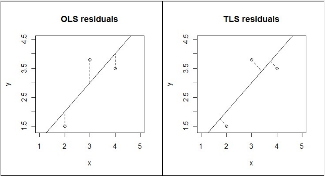
- 如上图，TLS 和 OLS 都是最小二乘拟合，只是在偏差评估上采取了不同的方式。
- 最小二乘法是一种较为简单的回归分析方法。
  The simplest example of a regression model is a straight line that passes through a set of points on a scatter plot.
  - Regression involves fitting a mathematical model to data.
  - Regression involves estimating the mathematical relationship between one variable called the response variable (or dependent variable), and one or more explanatory variables (or independent variables)
最常用的是 OLS（Ordinary Least Square，普通最小二乘法）：所选择的回归模型应该使所有观察值的残差平方和达到最小（如上图左）。
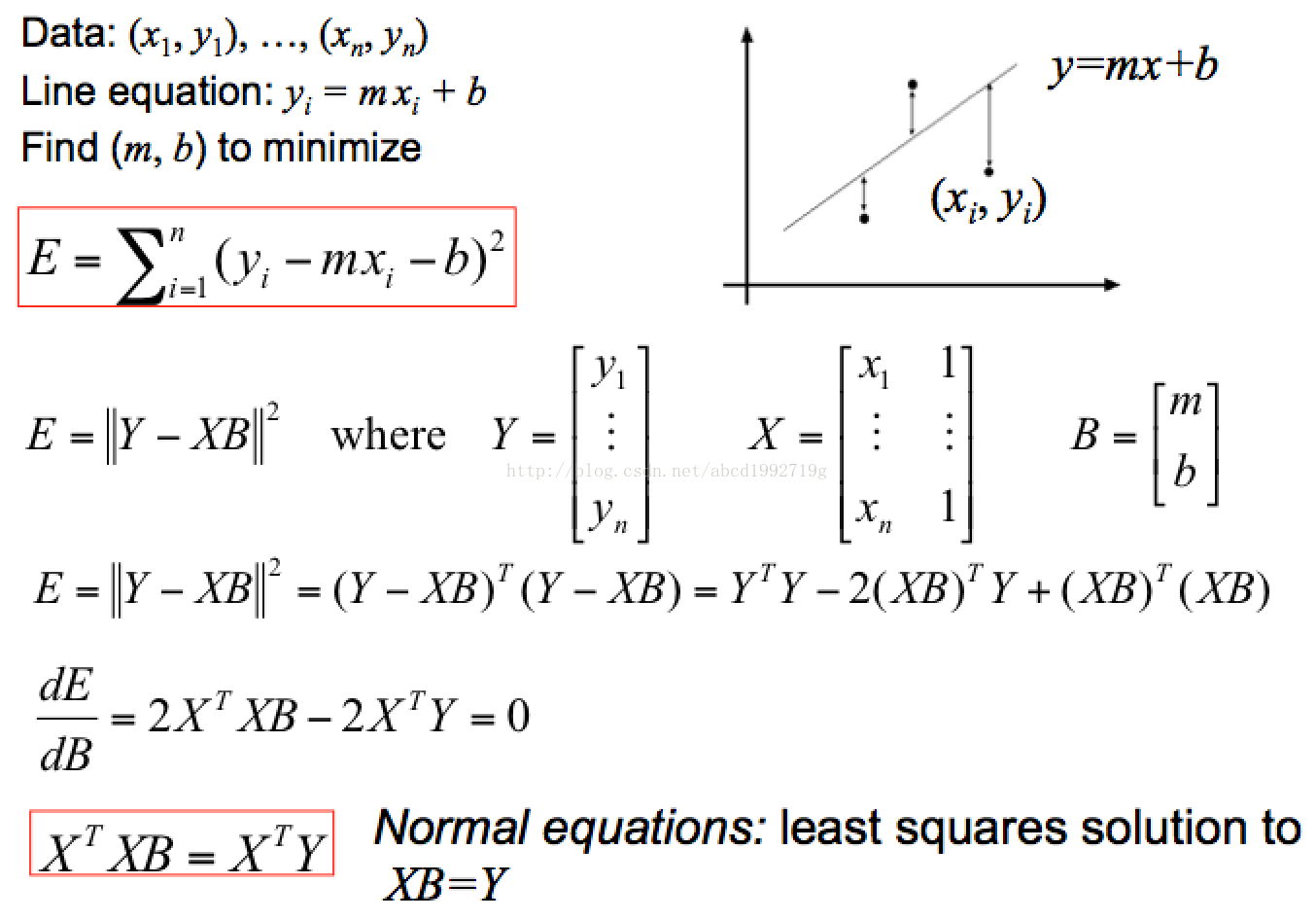
- 直接通过矩阵运算，容易得出：$B = (X^T X)^{-1}(X^T Y)$（拟合多项式：$y = b_0 + b_1 x + b_2 x^2 + … + b_k x^k$）

// Gary: O-Least-Square最小二乘拟合
Segment::LocalLine Segment::fitLocalLine(const std::list<Bin::MinZPoint> &points) {
  const unsigned int n_points = points.size();
  // 构造 X/Y 矩阵
  Eigen::MatrixXd X(n_points, 2);
  Eigen::VectorXd Y(n_points);
  unsigned int counter = 0;
  for (auto iter = points.begin(); iter != points.end(); ++iter) {
    X(counter, 0) = iter->d;
    X(counter, 1) = 1;
    Y(counter) = iter->z;
    ++counter;
  }
  // 计算 B
  const Eigen::MatrixXd X_t = X.transpose();
  const Eigen::VectorXd result = (X_t * X).inverse() * X_t * Y;
  LocalLine line_result;
  line_result.first = result(0);
  line_result.second = result(1);
  return line_result;
}

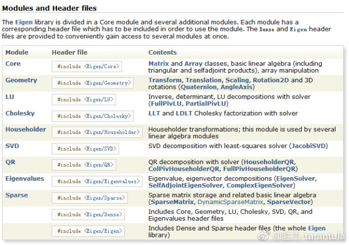
Eigen 是C++中可以用来调用并进行矩阵计算的一个库，里面封装了一些类。

通过解 $XB = Y$ 我们就能解出 $B = [m \space b]$：$$m = \frac{\sum x_i^2 \sum y_i - \sum x_i (\sum x_i y_i)}{n \sum x_i^2 - (\sum x_i)^2}$$ $$b = \frac{n \sum x_i \sum y_i - \sum x_i (\sum x_i y_i)}{n \sum x_i^2 - (\sum x_i)^2}$$

OrdinaryLeastSquare(const vector<double>& x, const vector<double>& y) {
        double t1=0, t2=0, t3=0, t4=0;  
        for(int i=0; i<x.size(); ++i)  { 
            t1 += x[i]*x[i];  
            t2 += x[i];  
            t3 += x[i]*y[i];  
            t4 += y[i];  
        }
        m = (t3*x.size() - t2*t4) / (t1*x.size() - t2*t2);
        b = (t1*t4 - t2*t3) / (t1*x.size() - t2*t2);
}

OLS 这种 least square 存在问题，比如针对垂直线段就不行，于是引入第二种 Total Least Square。
- 其中，$U = \begin{bmatrix} x_1 - \overline{x} & y_1 - \overline{y} \\ \vdots & \vdots \\ x_n - \overline{x} & y_n - \overline{y} \end{bmatrix}$；
- $\frac{dE}{dN} = \frac{d(N^T U^T U N)}{dN} = U^T U N + N^T U^T U$，因为 $U^T U$ 是一个对称矩阵（$U^T U = (U^T U)^T$），$U^T U N = N^T U^T U$，所以 $\frac{dE}{dN} = 2(U^T U)N$；
- 此外，$U^T U = \begin{bmatrix} \sum (x_i - \overline{x})^2 & \sum (x_i - \overline{x})(y_i - \overline{y}) \\ \sum (x_i - \overline{x})(y_i - \overline{y}) & \sum (y_i - \overline{y})^2 \end{bmatrix}$ 是关于 X、Y 的一个二阶矩（随机变量平方的期望）矩阵（second-moment matrix）；
- 二阶矩矩阵 $U^T U$ 的最小特征值对应的特征向量即为求解的 $N = [a \space b]$
  - 特征值 & 特征向量
    
    设 $A$ 为 n 阶矩阵（n × n），若存在常数 $λ$ 及 n 维非零向量 x（n × 1），使得 $Ax=λx$，则称 $λ$ 是矩阵 $A$ 的 特征值，$x$ 是 $A$ 属于特征值 $λ$ 的 特征向量。
  - $eig(U^T U) = [V, D]$，$V$ 是特征向量阵（每列为一个特征向量），$D$ 特征值对角阵 $\Longrightarrow$ 寻找 $D$ 中特征值最小的对角元素对应的特征向量即为 $U^T U$ 最小特征值对应的特征向量
    
    特征值分解：$U^T U = V D V^{-1}$
  - 通过 SVD（奇异值）求解
    - $SVD(A) = [U, S, V]$，即 $A = USV^T$
      
      ﹢其中 $U$ 是一个m*m的正交阵（Orthogonal matrix：满足 $U U^T = I$ 或者 $U^T U = I$ 的 n 阶方阵，其中 $I$ 为 n 阶单位阵），$S$ 是一个m*n的对角阵（Diagonal matrix：主对角线之外的元素皆为 0 的矩阵，对角线上的元素可以为 0 或其他值），对角线上的元素为 $A$ 的奇异值（Singular value），$V$ 是一个n*n的正交阵。$U$ 的 m 个列向量为 $A$ 的左奇异向量（Left singular vector），$V$ 的 n 个列向量为 $A$ 的右奇异向量（Right singular vector）。$S$ 完全由 $A$ 决定和 $U$、$V$ 无关；
      ﹢$A$ 的左奇异向量（$U$）是 $A A^T$ 的特征向量；$A$ 的右奇异向量是 $A^T A$ 的特征向量。
      ﹢$A$ 的非零奇异值是 $A^T A$ 特征值的平方根，同时也是 $A A^T$ 特征值的平方根。
    - 寻找 $S$ 中最小奇异值对应的 $V$ 的右奇异向量即为 $A^T A$ 最小特征值对应的特征向量。

#include <iostream>
#include <Eigen/Dense>
#include <Eigen/Eigenvalues>
 
using namespace Eigen;
using namespace std;
 
int main() {
    // Eigenvalue
    // typedef Matrix<int, 3, 3> Matrix3d
    Matrix3d A;
    A << 1, 2, 3, 4, 5, 6, 7, 8, 9;
    cout << "Here is a 3x3 matrix, A:" << endl << A << endl << endl;
    EigenSolver<Matrix3d> es(A.transpose() * A);
    // 对角矩阵，每一个对角线元素就是一个特征值，里面的特征值是由大到小排列的
    Matrix3d D = es.pseudoEigenvalueMatrix();
    // 特征向量（每一列）组成的矩阵
    Matrix3d V = es.pseudoEigenvectors();
    cout << "The eigenvalue matrix D is:" << endl << D << endl << endl;
    cout << "The eigenvector matrix V is:" << endl << V << endl << endl;
    // 特征值分解
    // cout << "Finally, V * D * V^(-1) = " << endl << V * D * V.inverse() << endl;
    // 特征值&特征向量
    cout << "min-eigenvector & min-eigenvalue" << endl;
    cout << " <1> The min-eigenvalue for A^T*A:" << endl << D(D.rows()-1, D.rows()-1) << endl;
    cout << " <2> The min-eigenvector for A^T*A:" << endl << V.col(V.cols()-1) << endl;
    cout << " <3> (A^T*A)*min-eigenvector =" << endl << (A.transpose()*A) * V.col(V.cols()-1) << endl;
    cout << " <4> min-eigenvalue*min-eigenvector =" << endl << D(D.rows()-1, D.rows()-1)*V.col(V.cols()-1) << endl << endl;
 
    // SVD
    // Eigen::ComputeThinV | Eigen::ComputeThinU
    Eigen::JacobiSVD<Eigen::Matrix3d> svd(A, Eigen::ComputeFullV | Eigen::ComputeFullU);
    Eigen::Matrix3d S = svd.singularValues().asDiagonal();
    //得到最小奇异值的位置
    Matrix3d::Index minColIdx;
    svd.singularValues().rowwise().sum().minCoeff(&minColIdx);
 
    cout << "The left singular vectors U is:" << endl << svd.matrixU() << endl << endl;
    cout << "The singular-value matrix S is:" << endl << S << endl << endl;
    cout << "The right singular vectors V is:" << endl << svd.matrixV() << endl << endl;
    cout << "The SVD: USV^T =" << endl << svd.matrixU()*S*svd.matrixV().transpose() << endl << endl;
 
    // 奇异值与特征值的关系
    cout << "The S^2 is:" << endl << S*S << endl << endl;
    cout << "The min-eigenvector for A^T*A:" << endl << svd.matrixV().col(minColIdx) << endl;
 
    return 0;
}

$d = a \overline{x} + b \overline{y}$；
最终得到的拟合直线：$y = -\frac{a}{b} x + \frac{d}{b}$

其他直线拟合方法

﹢基于 RANSAC(RANdom SAmple Consensus)（随机抽样一致）的直线拟合

王先荣：随机抽样一致性算法（RANSAC）

示例

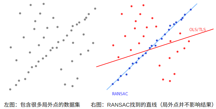
　（１）从一组观测数据中找出合适的2维拟合直线，观测数据中包含局内点和局外点，其中局内点近似的被直线所通过，而局外点远离于直线（如上图）；
　（２）简单的 最小二乘法 不能找到适应于局内点的直线，原因是最小二乘法尽量去适应包括局外点在内的所有点；RANSAC 能得出一个仅仅用局内点计算出模型，并且概率还足够高。
RANSAC　通过反复选择数据中的一组随机子集来达成目标（被选取的子集被假设为局内点），并用下述方法进行验证：
- ①：有一个模型适应于假设的局内点，即所有的未知参数都能从假设的局内点计算得出。
- ②：用①中得到的模型去测试所有的其它数据，如果某个点适用于估计的模型，认为它也是局内点。
- ③：如果有足够多的点被归类为假设的局内点，那么估计的模型就足够合理；用所有假设的局内点去重新估计模型，因为它仅仅被初始的假设局内点估计过，通过估计局内点与模型的错误率来评估模型。
- ④：①-③这个过程被重复执行固定的次数，每次产生的模型要么因为局内点太少而被舍弃，要么因为比现有的模型更好而被选用。

References

本文标题:[0025] Least Squares Line Fitting（最小二乘法直线拟合）

文章作者:Gary

发布时间:2017-07-21, 20:02:22

最后更新:2020-03-28, 12:37:22

原始链接:http://durant35.github.io/2017/07/21/Algorithms_LeastSquaresLineFitting/